Beamline Console
The beamline console is a command line enhanced IPython shell allowing users to configure and control beamline devices outside of the MxDC GUI. Commissioning activities such as scanning, plotting, fitting and scripting are all supported. As a normal python prompt, it allows traditional python scripts to be used in combination with device control and data-acquisition features provided by MxDC.
The beamline console includes a plot window which displays live data from currently executing scans, and results of some analysis after scans, such as curve-fitting.
The beamline console can be started using the blconsole command.
$ blconsole
For non-destructive testing and learning, a simulated console is available with a simulated beamline through the sim-console command.
$ blconsole
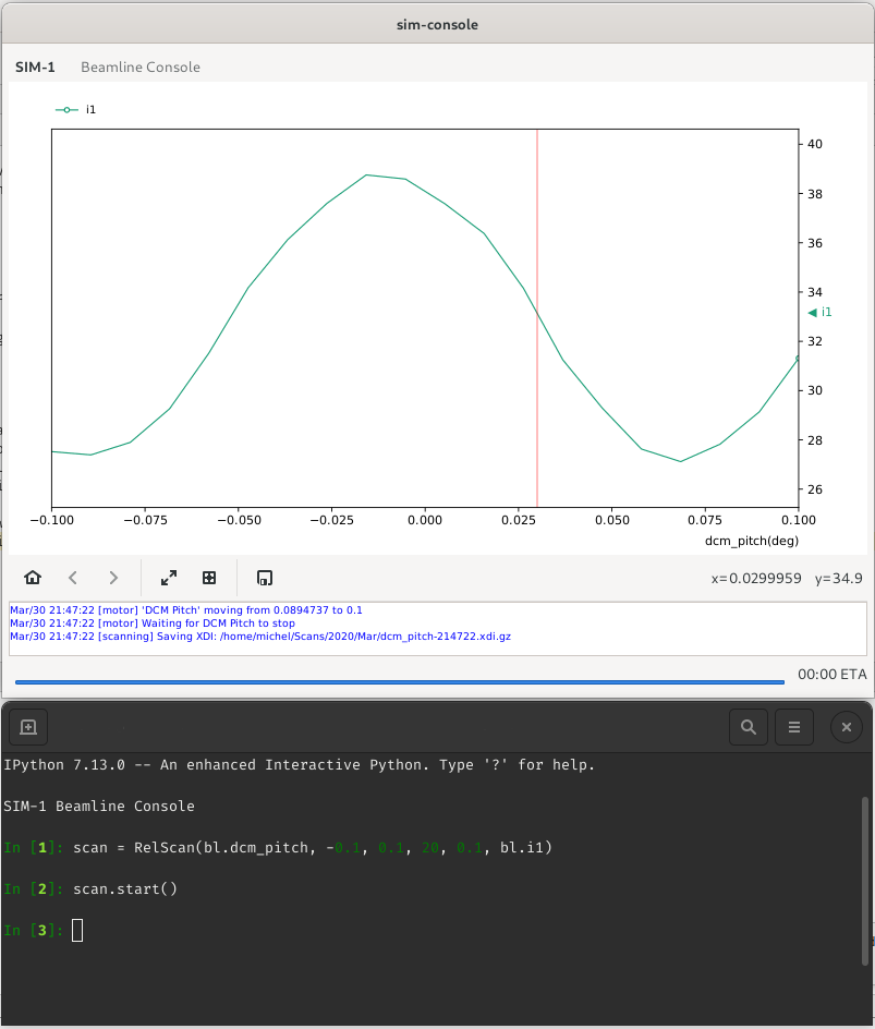
Screenshot of the Beamline Console showing the plot window and command prompt.
Default Environment
The following objects and classes are available in the default environment once the beamline console is launched.
bl - A reference to the beamline object. The devices registered will be available as attributes of this object.
plot - A reference to the plot controller.
fit - A fitting Manager object. This can be used to do curve fitting on the most recent scan data.
Various Scan types
|
An absolute scan of a single motor. |
|
Relative scan of a single motor. |
|
A Continuous scan of a single motor. |
|
Sequential Absolute scan of two motors. |
|
Sequential Relative scan of two motors. |
|
Absolute Step Grid scan of two motors. |
|
A Grid scan with Slewing of the inner motor (first). |
Warning
Avoid shadowing these names by assigning to them.
Performing Scans
To perform a scan, create a scan instance with the appropriate parameters and then call the start method to run the scan asynchronously. The plot window should update in realtime as the scan progresses.
>>> scan = RelScan(bl.dcm_pitch, -0.1, 0.1, 20, 0.1, bl.i1)
>>> scan.start()
While the scan is running, it can be stopped before it is complete
>>> scan.stop()
Sometimes, it is desirable to extend the scan range once the scan is complete, without destroying the previously
acquired data. In such cases, use the scan.extend() method as follows. The method takes a single parameter
which is the amount to extend the scan by in steps except for a SlewScan where the amount is the actual additional
travel range for the motor.
>>> scan.extend(10)   # 10 more steps for all other scan types
>>> scan.extend(2.5)  # 2.5 mm more for a Slew Scan
The introspection capabilities of IPython can be used to investigate objects. For example, to get help on required parameters for a specific type of scan, use the IPython help shortcut.
>>> SlewScan?
Init signature: SlewScan(m1, p1, p2, *counters, i0=None, speed=None)

Docstring:
A Continuous scan of a single motor.
:param m1: motor or positioner
:param p1: start position
:param p2: end position
:param counters: one or more counters
:param i0: reference counter
:param speed:  scan speed of m1
Fitting
To perform curve-fitting on the results of a scan, you can use the fit object as follows. Once the fit is complete, a fitted curve will be overlaid on the plot window and the fitted parameters will be returned. You can specify the data column to be used for fitting. The first column is selected by default if none is specified.
>>> fit.gaussian('i1')
{'ymax': 38.753925,
 'midp': -0.010566544083663901,
 'fwhm': 0.07076730539816214,
 'cema': -0.0009469308321938418,
 'midp_hist': -0.01071071087031274,
 'fwhm_hist': 0.08288288411793407,
 'ymax_hist': 38.75275534939397}
The following types of functions are available for fitting: gaussian(), lorentz(), voigt().
Saved Scan Data
Scan results are saved as GZip compressed XDI files like ~/Scans/YYYY/mmm/xxxxxx-HHMMSS.xdi.gz. These files can be displayed later using the plotxdi command provided with MxDC.
usage: plotxdi [-h] [-x X] [-y Y] file

Plot XDI data

positional arguments:
  file        File to plot

optional arguments:
  -h, --help  show this help message and exit
  -x X        X-axis column name
  -y Y        Y-axis column name